A few years back, the Washington Post published a visualization of Census data showing differences in housing in different large cities across the US. This was updated by Munson’s City, and both reports show the stunning abundance of single-family housing in American cities. Nationally, more than 60% of housing is detached single-family housing, and in more than half of the 50 largest US cities, single-family housing prevails as the dominant home type.
While cities such as New York and Boston are mostly made up of multi-family housing (in both cities, less than 20% of housing is single-family), data from Philadelphia show that it is truly a city of rowhomes. Philly and Baltimore are the only two cities analyzed with a majority of housing being single-family attached, or rowhomes. A prevalence of single-family housing in cities has implications in housing affordability, and many point to a lack of mid-density housing (or, the “Missing Middle”) as a threat to walkability and affordability.
Recognizing Philly as an outlier in the WaPo article, I decided to take a closer look at Philadelphia housing at the neighborhood scale. I re-created their visualization using US Census Bureau American Community Survey (2015-2019) data with Azavea’s definitions of Philly neighborhoods (though I realize these boundaries might be fluid and/or questionable to some). In the figure below, I show the 20 neighborhoods with the least single-family housing and the 20 neighborhoods with the most single-family housing. In between these two groups of extremes, you’ll find citywide numbers where, according to the most recent ACS numbers, about 65% of housing is single-family housing (but a relatively dense stock of single-family housing!).
Show code
# Housing type
# Jan 2021 -- Re-writing code from March 2019

library(tidyverse); library(sf); library(tidycensus); library(showtext)

#########################################################################
# Set up fonts

font_add_google('Merriweather')
font_add_google('Source Sans Pro', 'ssp')

showtext_auto()

font_theme <- theme(
  plot.title = element_text(family = 'Merriweather', face = 'bold'),
  plot.subtitle = element_text(family = 'ssp'),
  axis.text = element_text(family = 'ssp'),
  axis.title = element_text(family = 'ssp'),
  legend.text = element_text(family = 'ssp'),
  plot.caption = element_text(family = 'ssp', color = 'darkgray')
)
#########################################################################


census_api_key(Sys.getenv('census_api'))


# Get Azavea neighborhoods
neighborhoods <- st_read('https://raw.githubusercontent.com/azavea/geo-data/master/Neighborhoods_Philadelphia/Neighborhoods_Philadelphia.geojson')


# Get housing type data from ACS
housing_type <- get_acs(geography = 'block group',
                        table = 'B25024',
                        state = 'PA',
                        county = 'Philadelphia',
                        year = 2019,
                        geometry = T) %>%
  mutate(label = case_when(
    variable == 'B25024_001' ~ 'Total',
    variable == 'B25024_002' ~ 'Single family detached',
    variable == 'B25024_003' ~ 'Single family attached',
    variable == 'B25024_004' ~ '2 units',
    variable %in% c('B25024_005', 'B25024_006') ~ '3 to 9 units',
    variable == 'B25024_007' ~ '10 to 19 units',
    variable == 'B25024_008' ~ '20 to 49 units',
    variable == 'B25024_009' ~ '50+ units',
    variable == 'B25024_010' ~ 'Other'
  )) %>%
  st_transform(crs = st_crs(neighborhoods)) %>%
  st_join(neighborhoods, join = st_intersects) %>%
  group_by(mapname) %>%
  summarise(n = sum(estimate[label == 'Total'], na.rm = T),
            `Single family detached` = sum(estimate[label == 'Single family detached'], na.rm = T)/n,
            `Single family attached` = sum(estimate[label == 'Single family attached'], na.rm = T)/n,
            `2 units` = sum(estimate[label == '2 units'], na.rm = T)/n,
            `3 to 9 units` = sum(estimate[label == '3 to 9 units'], na.rm = T)/n,
            `10 to 19 units` = sum(estimate[label == '10 to 19 units'], na.rm = T)/n,
            `20 to 49 units` = sum(estimate[label == '20 to 49 units'], na.rm = T)/n,
            `50+ units` = sum(estimate[label == '50+ units'], na.rm = T)/n,
            Other = sum(estimate[label == 'Other'], na.rm = T)/n) %>%
  as_tibble() %>%
  mutate(total_p_sfh = `Single family detached` + `Single family attached`)


sfh_20_most <- housing_type %>%
  top_n(20, total_p_sfh)

sfh_20_least <- housing_type %>%
  top_n(-20, total_p_sfh)

citywide <- get_acs(geography = 'county',
                    table = 'B25024',
                    state = 'PA',
                    county = 'Philadelphia',
                    year = 2019) %>%
  mutate(label = case_when(
    variable == 'B25024_001' ~ 'Total',
    variable == 'B25024_002' ~ 'Single family detached',
    variable == 'B25024_003' ~ 'Single family attached',
    variable == 'B25024_004' ~ '2 units',
    variable %in% c('B25024_005', 'B25024_006') ~ '3 to 9 units',
    variable == 'B25024_007' ~ '10 to 19 units',
    variable == 'B25024_008' ~ '20 to 49 units',
    variable == 'B25024_009' ~ '50+ units',
    variable == 'B25024_010' ~ 'Other'
  )) %>%
  summarise(mapname = 'Citywide',
            n = sum(estimate[label == 'Total'], na.rm = T),
            `Single family detached` = sum(estimate[label == 'Single family detached'], na.rm = T)/n,
            `Single family attached` = sum(estimate[label == 'Single family attached'], na.rm = T)/n,
            `2 units` = sum(estimate[label == '2 units'], na.rm = T)/n,
            `3 to 9 units` = sum(estimate[label == '3 to 9 units'], na.rm = T)/n,
            `10 to 19 units` = sum(estimate[label == '10 to 19 units'], na.rm = T)/n,
            `20 to 49 units` = sum(estimate[label == '20 to 49 units'], na.rm = T)/n,
            `50+ units` = sum(estimate[label == '50+ units'], na.rm = T)/n,
            Other = sum(estimate[label == 'Other'], na.rm = T)/n) %>%
  mutate(total_p_sfh = `Single family detached` + `Single family attached`)


p_housing_types <- bind_rows(
  sfh_20_least,
  sfh_20_most,
  citywide
) %>%
  select(-n, -geometry) %>%
  pivot_longer(c(-mapname, -total_p_sfh), names_to = 'category', values_to = 'p_category') %>%
  mutate(category = factor(category,
                           levels = rev(c('Single family detached', 'Single family attached',
                                      '2 units', '3 to 9 units', '10 to 19 units',
                                      '20 to 49 units', '50+ units', 'Other'))))

# Kinda janky way to fix spacing in legend
# https://stackoverflow.com/questions/50883294/increasing-whitespace-between-legend-items-in-ggplot2/50885122
str_pad_custom <- function(labels){
  new_labels <- paste0(labels, '       ')
  return(new_labels)
}

my_palette <- rev(c('#e3ced3', '#aa82a8', '#6da18f', '#335b8e',
                '#b7dbdb', '#faed55', '#687e4f', '#424242'))
bold_citywide <- c(rep('plain', 20), 'bold.italic', rep('plain', 20))

# Make plot of housing types by neighborhood
p_housing_types %>%
  ggplot(aes(fill = category, y = p_category, x = reorder(mapname, -total_p_sfh))) +
  geom_bar(position = 'stack', stat = 'identity') +
  geom_hline(yintercept = c(0.25, 0.5, 0.75), linetype = 'dotted') +
  geom_hline(yintercept = 0) +
  labs(x = '', y = '', fill = '',
       title = 'What does housing look like in different Philly neighborhoods?',
       subtitle = 'Housing by Building Type',
       caption = 'Source: ACS 2015-2019 5-year estimates') +
  scale_y_continuous(expand = c(0, 0), breaks = c(0.25, 0.5, 0.75),
                     labels = c('25%', '50%', '75%')) +
  scale_fill_manual(values = my_palette, labels = str_pad_custom) +
  coord_flip() +
  theme(
    legend.position = 'bottom',
    plot.title = element_text(size = 15),
    plot.subtitle = element_text(size = 13),
    axis.text = element_text(size = 10.5),
    axis.text.y = element_text(face = bold_citywide),
    legend.spacing.x = unit(0.01, 'cm'),
    axis.ticks.x = element_line(linetype = 'dotted'),
    axis.ticks.y = element_blank(),
    panel.background = element_blank(),
    panel.grid = element_blank()
  ) +
  font_theme +
  guides(fill = guide_legend(nrow = 1, reverse = T))
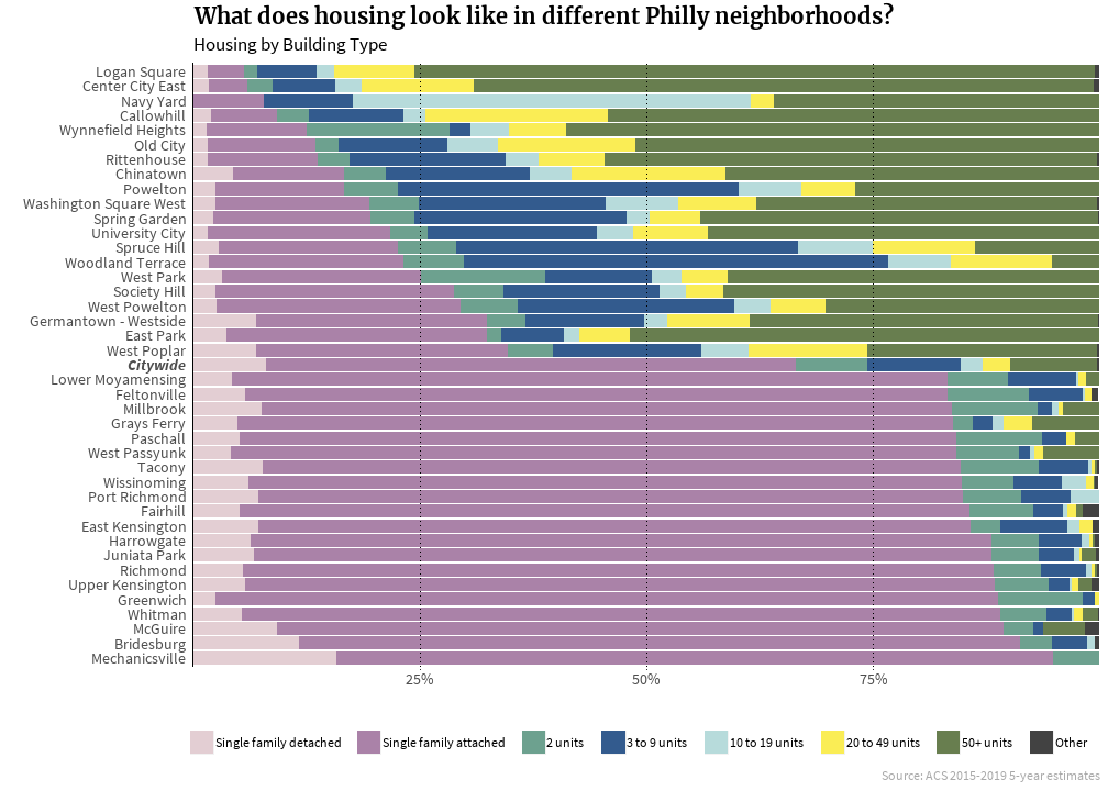
It’ll be interesting to take another look at this in a couple years, as I suspect data from some neighborhoods will reflect an emphasis on multi-family housing in development, and maybe some in the “missing middle.”